20260523 Workshop R

up::

1) Dados do IBGE

Pacotes usados:

• sidrar (tabelas do SIDRA-IBGE)
• rstudioapi: permite rodar todos os scripts dentro de algum diretório
• (data.table)

Funções importantes do sidrar:

• info_sidra: puxa informações de alguma tabela
  • E.g.: info_sidra(1612) puxa informações da tabela 1612 (Área plantada, área colhida, quantidade produzida, rendimento médio e valor da produção das lavouras temporárias)
• get_sidra: baixa os dados de uma dada tabela, com sintaxe de API
  • E.g.: get_sidra(/t/1612/n6/all/c81/2711/v/214/p/2024)
    • t (tabela): 1612;
    • n6 (Geografia, 6=Microrregião): todas;
    • c81 (“Classification category”) (classific_category$c81 = Produto das lavouras temporárias (34):) = 2711 Milho (em grão);
    • v: variável (214, neste caso);
    • p(eriod): 2024

Dá pra usar os parâmetros da função get_sidra para não usar sintaxe de API. No caso acima ficaria

get_sidra(
  1612,
  variable=214,
  period=c("2024"),
  geo="City",
  classific=c("c81"),
  category=list("2711")
)

Dá pra especificar (onde for possível) períodos de tempo, e.g. 202401-202412.¹

2) Dados climáticos

Site NASA POWER: NASA POWER | Homepage.

Funções puxadas do repositório EnvRtype:

source('https://raw.githubusercontent.com/allogamous/EnvRtype/master/R/AtmosphericPAram.R')
source('https://raw.githubusercontent.com/allogamous/EnvRtype/master/R/SradPARAM.R')
source('https://raw.githubusercontent.com/allogamous/EnvRtype/master/R/SupportFUnction.R')
source('https://raw.githubusercontent.com/allogamous/EnvRtype/master/R/EnvTyping.R')
source('https://raw.githubusercontent.com/allogamous/EnvRtype/master/R/Wmatrix.R')
source('https://raw.githubusercontent.com/allogamous/EnvRtype/master/R/covfromraster.R')
source('https://raw.githubusercontent.com/allogamous/EnvRtype/master/R/envKernel.R')
source('https://raw.githubusercontent.com/allogamous/EnvRtype/master/R/gdd.R')
source('https://raw.githubusercontent.com/allogamous/EnvRtype/master/R/getGEenriched.R')
source('https://raw.githubusercontent.com/allogamous/EnvRtype/master/R/get_weather_gis.R')
source('https://raw.githubusercontent.com/allogamous/EnvRtype/master/R/processWTH.R')
source('https://raw.githubusercontent.com/allogamous/EnvRtype/master/R/met_kernel_model.R')
source('https://raw.githubusercontent.com/allogamous/EnvRtype/master/R/summary_weather.R')
source('https://raw.githubusercontent.com/allogamous/EnvRtype/master/R/plot_panel.R')

Puxando informações de clima:

local <- "Sorriso_MT_BRA"
lat = -12.5425
lon = -55.7211
data.inicial = as.Date("1/1/2010",format='%m/%d/%Y')
data.final = as.Date(Sys.Date(),format='%m/%d/%Y')
  
dados_climaticos <- get_weather(env.id = local, 
                                lat = lat,
                                lon = lon,
                                start.day = data.inicial,
                                end.day = data.final)

As colunas são (cf. EnvRtype/man/get_weather.Rd at master · allogamous/EnvRtype · GitHub)

The available variables are (from NASAPOWER & Computed):
\itemize{
 \item T2M: Temperature at 2 Meters. C
 \item T2M_MAX: Maximum Temperature at 2 Meters, C
 \item T2M_MIN: Minimum Temperature at 2 Meters, C
 \item PRECTOT: Precipitation (mm)
 \item WS2M: Wind Speed at 2 Meters, m/s
 \item RH2M: Relative Humidity at 2 Meters, percentage
 \item QV2M: Specific Humidity, the ratio of the mass of water vapor to the total mass of air at 2 meters (kg water/kg total air).
 \item T2MDEW: Dew/Frost Point at 2 Meters, C
 \item ALLSKY_SFC_LW_DWN: Downward Thermal Infrared (Longwave) Radiative Flux
 \item ALLSKY_SFC_SW_DWN: All Sky Insolation Incident on a Horizontal Surface
 \item ALLSKY_SFC_SW_DNI All Sky Surface Shortwave Downward Direct Normal Irradiance
 \item ALLSKY_SFC_UVA: All Sky Surface Ultraviolet A (315nm-400nm)  Irradiance
 \item ALLSKY_SFC_UVB: All Sky Surface Ultraviolet B (280nm-315nm)  Irradiance
 \item ALLSKY_SFC_PAR_TOT: All Sky Surface Photosynthetically Active Radiation (PAR) Total
 \item FROST_DAYS: If it was a frost day (temperature less than 0C or 32F)
 \item GWETROOT: Root Zone Soil Wetness (layer from 0 to 100cm),ranging from 0 (water-free soil) to 1 (completely saturated soil).
 \item GWETTOP: Surface Soil Wetness (layer from 0 to 5cm),ranging from 0 (water-free soil) to 1 (completely saturated soil).
 \item EVPTRNS: Evapotranspiration energy flux at the surface of the earth.
 \item P-ETP: Computed difference between preciptation and evapotranspiration.
 \item VPD: Vapour pressure deficit (kPa), computed from T2MDEW,T2M_MAX and T2M_MIN
 \item N: Photoperiod (in h), computed from latitude and julian day (day of the year)
 \item n: number of sunny hours in the day for a clear sky (no clouds)
 \item RTA: Radiation on the top of the atmosphere, computed from latitude and julian day (day of the year)
 \item TH1: Temperature-Humidity Index by NRC 1971
 \item TH2: Temperature-Humidity Index by Yousef 1985
 \item PAR_TEMP: computed ratio between ALLSKY_SFC_PAR_TOT and  T2M
}

Vale checar no futuro dados do CPTEC/INPE: GitHub - rpradosiqueira/cptec: An R interface to the CPTEC/INPE API · GitHub (Inclusive, do mesmo GOAT que criou o sidrar!).

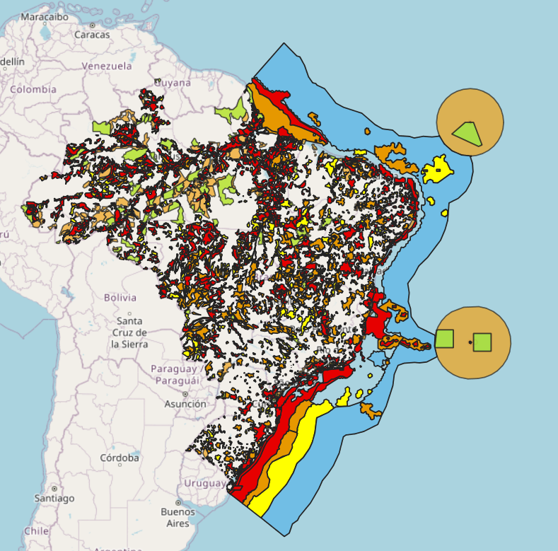
Outra joia é o visualizador geográfico do INDE: Visualizador da INDE - Infraestrutura Nacional de Dados Espaciais. IMPRESSIONANTE! E.g. áreas de conservação (ICM-Bio):

3) Importando dados de investimento

Meio precário: um exemplo

empresa <- "VALE3"
url <- paste("https://www.fundamentus.com.br/detalhes.php?papel=",empresa, sep="")

Mencionaram Brazil Data Cube Documentation — Brazil Data Cube, BIG – Brazil Data Cube – Plataforma para Análise e Visualização de Grandes Volumes de Dados Geoespaciais.

4) Imagens de satélite

# Exemplo com imagem Sentinel-2 ou Landsat.
# Cada arquivo representa uma banda espectral.

blue  <- rast("B02.tiff")   # Banda azul
green <- rast("B03.tiff")   # Banda verde
red   <- rast("B04.tiff")   # Banda vermelha
nir   <- rast("B08.tiff")   # Infravermelho próximo

# Criar um objeto com várias bandas juntas
img <- c(blue, green, red, nir)
names(img) <- c("Blue", "Green", "Red", "NIR")

# Composição RGB verdadeira
# Red = banda vermelha
# Green = banda verde
# Blue = banda azul
plotRGB(img,
        r = 3, # terceira variável da lista
        g = 2, # etc
        b = 1,
        stretch = "lin",
        main = "Composição RGB Verdadeira")
        

# Composição falsa cor
# Muito usada para vegetação
# NIR aparece em vermelho
plotRGB(img,
        r = 4,
        g = 3,
        b = 2,
        stretch = "lin",
        main = "Composição Falsa Cor")

Cálculo de NDVI (NIR = Near InfraRed):

# Valores próximos de 1 indicam vegetação mais vigorosa.
# Valores próximos de 0 indicam solo exposto ou vegetação fraca.
# Valores negativos podem indicar água, sombra ou áreas não vegetadas.
NDVI = (NIR - Red) / (NIR + Red)

Mencionaram sobre o CBERS (China-Brazil Earth Resources Satellite), p. ex. Satélite CBERS-4A – Dados Geoespaciais.

Parece dar pra puxar daqui INPE :: Catálogo de Imagens, embora pareça requerer cadastro (grátis, nonetheless).

5) Criação de mapas

Aula INTEIRA arrumando erro que não estava lendo mapa_municipios…

6) Workflow de modelos de ML

Resolvendo a bosta do erro do geobr (pelo menos deu certo).

7) Criando aplicativos no R (Shiny!)

Todo aplicativo em Shiny possui ao menos ui e server.

O ui monta uma página fluidPage em vários fluidRow’s e colunas. Seu formato é feito em HTML.

Os servidores possuem variáveis reativas (reactiveVal) — que serão as variáveis atualizáveis dentro do ui — e eventos observeEvent’s — que podem (ou não) mudar tais variáveis.

Para que apareçam novas coisas na página, pode-se usar

• renderPrint: mero print
• renderUI: alteração da UI
• renderText: welp…
• renderDT: Data Table

Variáveis reativas sempre aparecem da forma var_reativa().

Boas ideias podem vir de Shiny for R Gallery.

Uma ideia que quero ver algum dia é um gráfico do Brasil com as produtividades (Soja, Milho, Trigo) vide SIDRA/IBGE. Quem sabe algo dos dados pecuários também.

Dá pra publicar Shiny apps em shinyapps.io.

8) Relatórios automáticos no R

Relatório é algum arquivo __.qmd, com YAML e corpo do texto após.

knitr::kable(variavel) gera uma visualização de variavel. Por exemplo,

	```{r}
	kpis <- data.frame(
	  Indicador = c("Número de linhas", "Número de colunas"),
	  Valor = c(
	    scales::comma(nrow(dados)),
	    scales::comma(ncol(dados))
	  )
	)
	
	knitr::kable(kpis, align = "c")
	```

---

Referências

Workshop Aplicando R no Mundo Real - YouTube

Footnotes

1. No caso de tabelas do PAM, informações são somente por ano. ↩